GENERATING A GREEN BAND FOR GOES-16

GOES-16 and GOES-17 have no green band so one has to be created from the blue, red, and near-infrared channels. But no amount of simple blending of those channels will produce a truly accurate synthetic green band so additional processing—e.g. a look up table (LUT)—is usually necessary to further compensate.

For demonstration purposes I'll be using mostly Himawari-8 imagery in this post. Himawari and GOES share the same imager with reasonably similar blue, red, and near-infrared bands. The big difference, of course, is Himawari includes a visible wavelength green filter (though at a wavelength that is not ideal for true color). GOES prioritizes a unique near-infrared filter in place of a green one.

By combining blue, red, and near-infrared channels Himawari will produce approximately what GOES is capable of. This can then be compared to Himawari imagery using its RGB filters (with a little near-infrared added to boost the vegetation signal).

Here is a commonly cited GOES synthetic green channel formula:

# Typical pseudo-green channel formula
# B: blue band
# R: red band
# I: near-infrared band
pseudo_G = B * 0.45706946 + R * 0.48358168 + I * 0.06038137

Here is how Australia would look using this formula:

Australia with a typical GOES synthetic green band (left) and in true color (right).

The true-color image is on the right for comparison. The colors in the left panel are what pass for "true color" for much of the non-NOAA/NASA GOES imagery seen online. To be fair, this is the most basic and accessible level of color generation used.

Ideally I would like to not have to do custom editing in an external program like GIMP or Photoshop. The goal is for anyone to be able to easily reproduce my results. Figuring out how to achieve this automatically in a Python script is what I'm working on now.

PREVIEW
Here is a work-in-progress image from the previous post using my current Python script and without any retouching:

GOES-16 satellite view of Earth using a Python script to generate the missing green band.

I'm still not satisfied with how the deserts of the United States and Mexico appear under certain sun angles (see Limitations below).

In the example above the deserts appear as a low-saturation yellow compared to the overall image but they are actually gray or very slightly blue when seen in isolation. That makes them exceedingly difficult to separate from other blue pixels for targeted adjustment! Shallow water that should be turquoise presents the same challenges.

PROGRESS
By masking pixels within a certain hue range I have been able to bring their color closer to what they should be. With Himawari-8 data I can make a pseudo-green channel and compare the results to true color as seen here:

Himawari-8 in synthetic green (left) vs true color (right). Himawari-8: Satellite image originally processed by the Bureau of Meteorology from the geostationary satellite Himawari-8 operated by the Japan Meteorological Agency.

[Update: April 27, 2020] I was able to eliminate the masking and hue rotation stage and use only channel blending of the existing bands.

import numpy as np
import cv2

# New pseudo-green channel formula
# This is still experimental!
# 
# Blend the B channel and R channel
G_base = cv2.addWeighted(B, 0.38, R, 0.62, 0)

# Use the I channel to lighten G_base using np.maximum
# This will increase the vegetation signal
G_veg = cv2.addWeighted(G_base, 0.97, np.maximum(G_base, I), 0.03, 0)

# Blend the B channel to decrease the signal
# in predominantly red/orange soil regions
G_soil = new_G = cv2.addWeighted(G_veg, 0.41, np.minimum(G_veg, B), 0.59, 0)

The script then merges the channels to the BGR [blue/green/red] color model and then converts it to the HLS [hue/lightness/saturation] color model where a tone curve is applied to the lightness channel. This will greatly boost the saturation which is what we want.

# Create a "true color" BGR image
img = cv2.merge((B, new_G, R))

# Convert BGR to HLS
hls = cv2.cvtColor(img, cv2.COLOR_BGR2HLS)

# Split image to HLS components
h, l, s = cv2.split(hls)

# Adjust the tone curve
# function: y = (x^b(x+1-xa))^1/c
# https://www.desmos.com/calculator/wf7oex5edi
a = 1.85
b = 0.90
c = 1.90

new_l = np.power(np.power(l, b * (l + 1 - (l * a))), 1/c)

# Merge to HLS
new_img = cv2.merge((h, new_l, s))

# Convert to BGR
img = cv2.cvtColor(new_img, cv2.COLOR_HLS2BGR)

Here is the result over the course of one day:

Earth at two hour intervals as acquired by Himawari-8 on August 15-16, 2019. An experimental green channel formula for use with GOES has been used in place of the green band.

Note how Australia still lacks some of the subtle color variation within the orange hue range relative to true color. As an aside, also note the extreme phase lightening as Earth approaches solar noon! This is actually a problem and is not quite how an observer would perceive it.

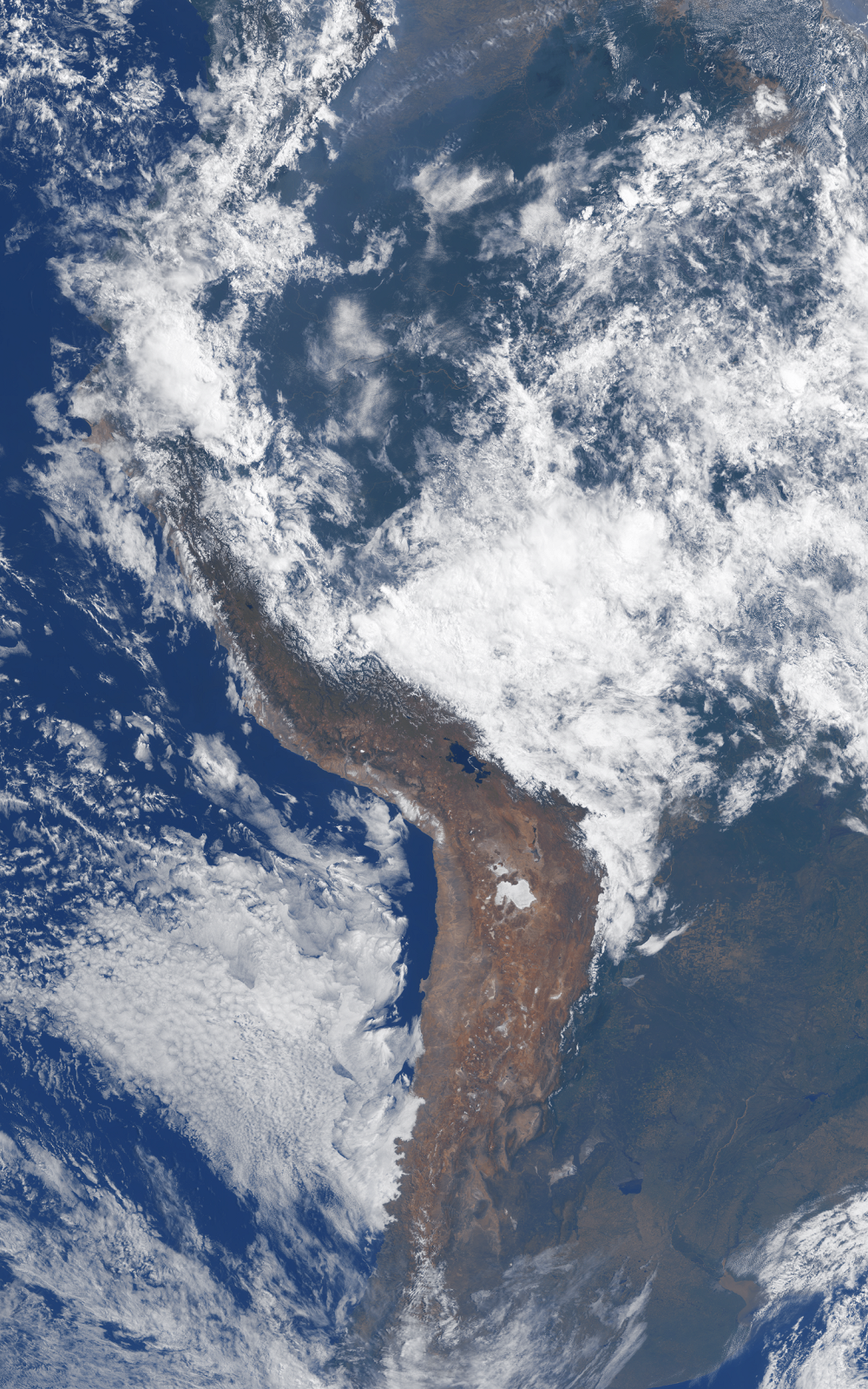
Here is the view from GOES-17 using the current Python script:

The vast expanse of the Pacific Ocean as seen from GOES-17 on May 2, 2020 at 20:00 UTC.

LIMITATIONS
As the incident angle of light increases the issue with orange soils becomes even more apparent.

As the angle of incidence increases the limitations of pseudo green (left) compared to true color (right) become obvious.

In the bidirectional reflectance factor (BRF) image above Australia once again loses its reddish appearance (left) just as it did with the old pseudo green formula. This problem worsens not only as the view approaches the limb and terminator but even with seasonal changes.

ADDING A LOOK UP TABLE (LUT)
A generated LUT made by comparing true color and pseudo true color images can greatly reduce the differences in soils but it is less successful with turquoise water.

With a LUT applied, soils look much better but turquoise water remains too blue.

I assume this is because GIMP uses a weighted average of similar blue pixels for the LUT. Most of Earth is blue and it would not be useful to make it all cyan just for the tiny fraction of visible shallow water.

The GOES-16 image in the Preview section was made using the same Python script that was used for the first Himawari example in the Progress section above. Applying the LUT to GOES-16 returns this result:

GOES-16 with a LUT applied derived from Himawari-8.

I'm exploring the practicality of using LUTs in Python scripts but it seems like this would be far from trivial to implement. A single LUT would not work for all lighting conditions, for example. And if weighting is used, the prominence of Australia in Himawari may skew deserts too orange in other regions.

Conversely, there is a dearth of unclouded, heavily forested areas near satellite nadir in Himawari necessary for GOES-16.

Ideally, both solar incident and satellite view angles would be used with multiple/dynamic LUTs generated for a range of lighting and spatial geometries.

ATMOSPHERIC CORRECTION
Much of GOES imagery online has had atmospheric correction applied. Atmospheric correction reduces the attenuating/blueing effects of the atmosphere and makes isolating and correcting shallow water color easier.

Since I'm more interested in Earth as a human observer in space would view it I don't have that option.

CREDIT
Australian Bureau of Meteorology http://www.bom.gov.au/metadata/19115/ANZCW0503900400
Japan Meteorological Agency
NASA
NOAA

This work is licensed under a Creative Commons Attribution-ShareAlike 4.0 International License.